Assessing Concordance in Post-operative Knee Implant Position Analysis Between Automated Image Analysis Algorithm and Human Radiologists

Click here : https://joeipub.com/learning

Introduction

Identifying post-operative implant position is essential for the analysis of orthopedic implants in knee replacement surgery. These measurements can provide quantitative data on surgical execution and can provide insights on different surgical methods, such as conventional, navigation and robotic-assisted.

Unfortunately, making these measurements (for example, by identifying landmarks in CT images) is time-consuming and requires trained medical specialists. Even with trained professionals we observe differences in intra- and inter-observer reliability for certain implant position parameters (Miura et al. 2018; Yoshino et al. 2019).

Most post-operative assessments rely on plain radiographs, their accessibility, low cost and low radiation dose makes it a mainstay in routine clinical practice. However many factors such as leg rotation, flexion and magnification errors can affect these measurements and can lead to inaccuracies (Brouwer et al. 2007; Holme et al. 2011a; Radtke, Becher, Noll, et al. 2010; Jamali et al. 2017).

Additionally, it is not possible to measure the 3D position & orientation of an implant from a 2D radiograph. Implant rotation can be assessed using two-dimensional computed tomography (2D-CT) (Berger et al. 1998; Jazrawi et al. 2000). While this method provides 3D data, 2D slices may lead to inaccuracies due to leg orientation during scanning influencing the location of anatomical landmarks (Slevin et al. 2018).

To assess post-surgical implant position accuracy, it is essential to establish a reproducible and accurate evaluation method. Unfortunately, the reproducibility and evaluation method for post-operative alignment is often not validated (De Valk, Noorduyn, and Mutsaerts 2016). Recently the use of automated 3D measurement based on CT scans shows promise in deriving implant position values more reproducibly (Slevin et al. 2018; Watanabe, Akagi, Shiko, et al. 2021; Hirschmann et al. 2011; Cerquiglini, Henckel, Hothi, et al. 2018).

Stryker has developed a methodology for locating implants in CT images where we automate all stages of the process, thus eliminating human error and variability. Using a novel approach of Bayesian hierarchical modeling, the authors aimed to determine if concordance exists (defined as a three-way agreement between the two radiologists and the algorithm). Therefore, the model will evaluate corroboration between both the radiologists and the algorithm.

Material and Methods

Patients and surgical technique

We collected CT scans from patients undergoing TKA surgery in the RCT (NCT03566875) who received primary TKA between March and December 2018. In total 60 patients were enrolled in this study, and we received consent from 48 patients to use their data. Patient demographic data, including sex and age, were not provided to the authors since they were considered unnecessary for this study.

The surgeons used the Triathlon™ Knee (Stryker, Kalamazoo, Michigan, USA) for all cases with cement fixation. Our dataset has a mixture of robotic-assisted and manual TKA. All patients received a pre-operative CT scan and underwent a post-operative CT scan 7 days after surgery. Both scans were subject to the Stryker Mako CT protocol, which took 1 mm slices at the knee, and lower resolution images at 2 mm slices at the hip and ankle.

Automated Image Analysis

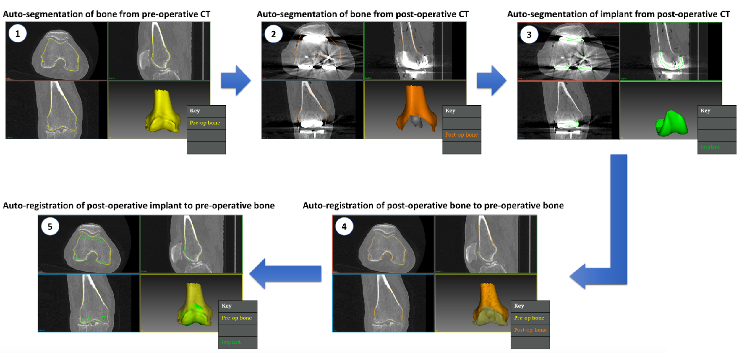
CT scans were analysed to compare post-operative implant position to the pre-operative planned position. The analysis workflow (see Figure 1) was performed with a custom automatic segmentation and automatic registration process. Step 1 involved automatic segmentation of the femur and tibia in the pre-operative CT image. Secondly, the bones were automatically segmented in the post-operative CT image. Segmentation of bones can be difficult in a post-operative image for three reasons: (1) portions of the patient’s bone have been removed during surgery; (2) identifying bright voxels and edges corresponding to the implant itself; and (3) scattering artefacts due to the presence of metal in the image. A specialised version of the automatic segmentation process was developed to overcome all three challenges. After segmenting the bones, the automated segmentation tool was then used to segment the implant. Segmentation of the implant can also be difficult, due to scatter and other image artefacts resulting from the metal of the implants. To overcome these challenges, a database of implant designs was used to select a 3D model of the exact design and size of the implant used in each surgical case, and a specialised automatic segmentation model based on that implant was employed.

Figure 1.Description of workflow to analyze surgical implant placement based on pre-operative and post-operative CT scans. An automated segmentation and automated registration process was developed and specialized for this study.

After segmentation was completed, an automated registration process was used to align the post-operative bone with the pre-operative bone. The executed implant placement was then compared with the intra-operative planned implant position and the difference between these two plans was calculated to provide the error in implant placement.

Manual Image Analysis

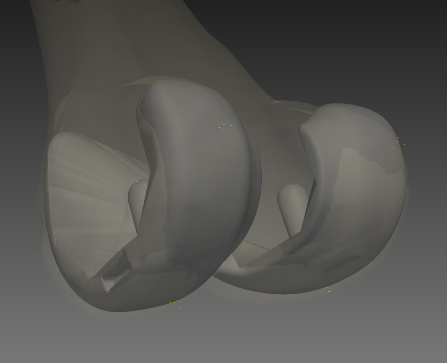
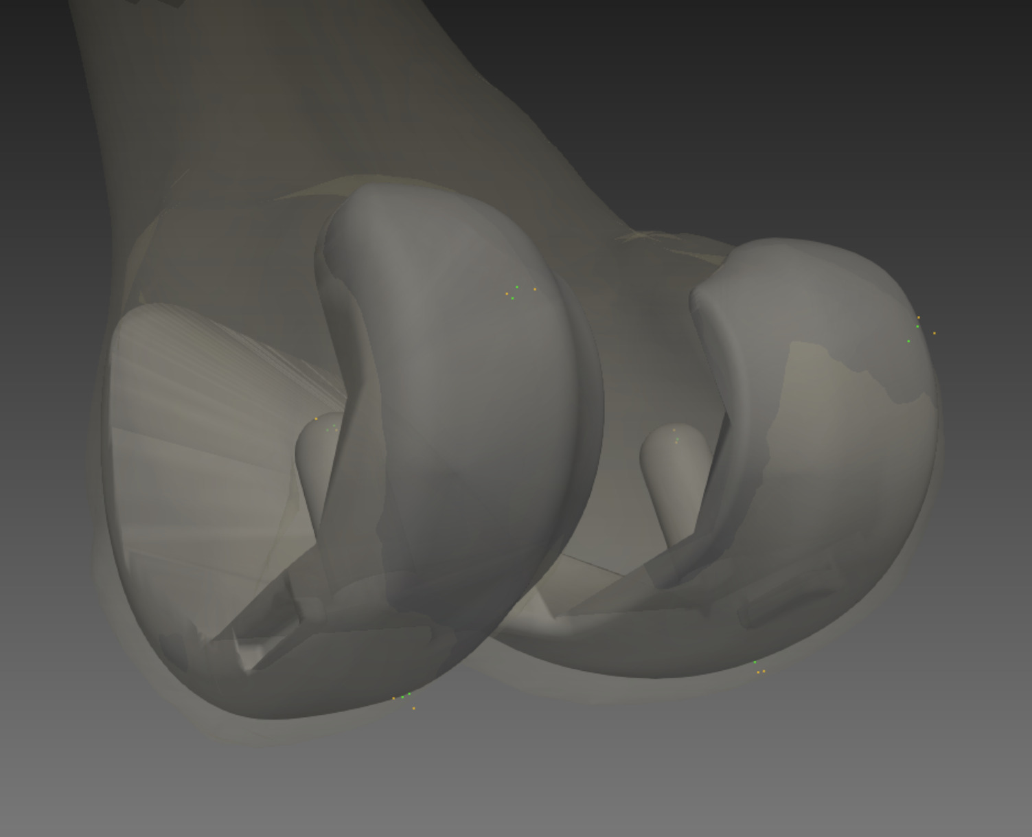
Two consultant radiologists independently evaluated all 48 patients and repeated their measurements twice. For each patient the radiologists marked several landmarks from CT images. The landmarks used to compute implant axes in 3D space are shown in Table 1. A 3D illustration of these landmarks on the femoral component is shown in Figure 2, where each colour represents a different radiologist.

Figure 2.Illustration of femoral landmarks taken by two radiologists (green: radiologist 1, orange: radiologist 2) in 3D.

The medial-lateral femoral axis (x-axis) was defined as the average between the lines generated by landmarks 1 & 2, 3 & 4, and 5 & 6. Rotation about the x-axis will be the flexion/extension angle. The superior-inferior axis (z-axis) was defined as the average between lines generated by landmarks 3 & 5, and 4 & 6. Rotation about the z-axis is the internal/external angle. The anterior-posterior axis (y-axis) was the cross product of the two previously generated axes and the rotation about the y-axis is the varus/valgus angle.

Similarly the tibial medial-lateral axis was defined as the average lines generated by landmarks 7 & 8, and 9 & 10. The anterior-posterior line was defined from the landmarks 11 & 12, and the superior-inferior axes were the cross product of the two previously generated axes.

Theory/Calculation

Bayesian Statistical Analysis

We employed a hierarchical Bayesian model to address the concordance dilemma, aiming to determine whether the landmarks identified by two radiologists were indistinguishable from each other and from our algorithm (Gelman et al. 2013).

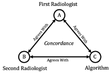
To explain concordance, consider the graph in Figure 3 where each node represents an agent in the experiment. We want to test if:

1. The landmarks identified by two radiologists (nodes A and B) are indistinguishable.

2. Radiologist’s landmarks match those of an algorithm (node C).

3. All three agents (both radiologists and the algorithm) produce indistinguishable results.

Figure 3.Graph network demonstrating the problem of concordance

We’re testing whether there’s any detectable difference among all agents in the network (Linde et al. 2021).

Bayesian hierarchical models, also known as multilevel models, are probabilistic frameworks used to estimate parameters across different groups. These models account for both the individual characteristics of each group and the similarities between them, enabling more accurate predictions. By sharing information across groups, they help prevent overfitting (overly complex models) or underfitting (overly simple models). A key feature of hierarchical models is shrinkage, which naturally regularises estimates by pulling extreme values or results from small groups toward the overall average, thereby reducing the influence of outliers or sparse data (Lustig et al. 2021).

For this research, the groups were stratified into two levels: patient and radiologist. Where j=2 for radiologists and k=48 for total knees. The hierarchical model architecture lends itself well to the data, given that there are multiple, repeated observations per doctor per patient, which would violate the assumption of independence for many frequentist statistical tests. The full model structure and equations are detailed in Appendix A.

One of the advantages of Bayesian methods is that they afford the researcher multiple options in interpreting results that extend and, in many cases, surpass the null hypothesis significance testing framework. By comparison, Bayesian methods allow the decision criteria to be created to reject or accept the null hypothesis. These options map well to this research objective, as the goal is to accept the null hypothesis per the concordance research objective and aligns with Bayesian principles by:

1. Incorporating uncertainty explicitly in the analysis, providing a richer understanding of the parameter estimates.

2. Facilitating hypothesis testing in a Bayesian framework through the use of probabilistic statements about parameters rather than relying solely on p-values.

3. Enhancing interpretability of the results by examining the relationship between parameters and their joint effects on outcomes.

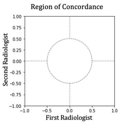
To evaluate concordance, we applied a Region of Practical Equivalence (ROPE) (Kruschke 2018), establishing a boundary of ±0.5 degrees. If more than 95% of the joint posterior distribution falls within this boundary, concordance is achieved. Otherwise, concordance is rejected. Figure 4 illustrates this decision process.

Figure 4.Demonstration of the Region of Practical Equivalence or ROPE of concordance. The ROPE is essentially mapped from a one-dimensional to two-dimensional space.

Results

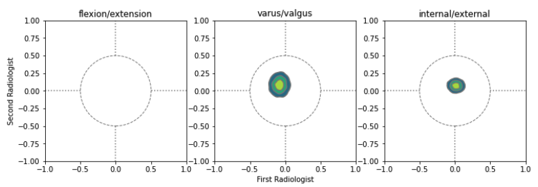
The models were fit independently for the flexion/extension, varus/valgus, and internal/external angles for both the tibia and femur using the Metropolis-Hastings algorithm, with 3000 samples generated and 1000 subsequently discarded during the initial sampling process to promote chain convergence and optimal mixing. All models displayed good mixing and convergence. Table 2 represents the model output related to the radiologists’ common effects. Figures 5 and 6 show the joint distribution plots of the posteriors for the common effects mapped to the concordance decision rule.

Figure 5.Posterior plots for the femur, the contours on the plot represent one standard deviation from the mean of the posterior.

Figure 6.Posterior plots for the tibia, the contours on the plot represent one standard deviation from the mean of the posterior.

In this paper, positive values of flexion/extension indicate more flexed, positive values of varus/valgus more varus, and positive values of internal/external rotation more internal.

The above figures (5, 6) show the 95% HDI for the joint posterior distributions mapped to the concordance decision rule. The plots demonstrate concordance for the femur of varus/valgus and internal external. By comparison, concordance only exists for varus/valgus for the tibia. When reviewing the posterior distributions for the tibia, it is apparent that the distributions are much broader when compared to the femur. Given that the data points are the same for both anatomical regions, the broader joint posterior distributions are driven by larger variances within the data and between the radiologists. Much of this variance can also be assumed to be driven by the inherent challenges of identifying landmarks for the tibia, which will be addressed in the Discussion.

To gain intuition as to how the model functions and how the concordance decision rule can be interpreted, we can draw an example from the flexion/extension of the femur. Reviewing Figure 5, it can be concluded that concordance was not achieved for this angle. However, further insight can be illuminated upon closer inspection of the individual posterior distributions for both radiologists, as shown in Figure 7, which displays the individual posterior plots for the femur flexion/extension for the fixed effects of both radiologists. The plot demonstrates the posterior distributions, the mean of the posterior distribution labelled in black, the percentage of the distribution falling above or below the posterior mean in orange, and the percentage of the posterior falling within the ROPE in green.

Figure 7.Individual posterior plots for the femur flexion/extension for the fixed effects of both radiologists. The plot displays the mean of the posterior in black, the observed mean value, and the percentage of the distribution above and below the mean in orange, and the ROPE in green, along with the percentage of the distribution that includes the ROPE boundary.

The posterior distribution on the left demonstrates that the first radiologist disagreed with the algorithm, as shown by the entire distribution excluding the ROPE boundaries. By comparison, the distribution on the right shows that approximately 39% of the posterior contains the ROPE, meaning that a conclusion must be withheld for this radiologist. It is, therefore, acceptable to conclude that in this instance, not only did the radiologists disagree with the algorithm but with each other as well as neither posterior cross the barrier of the concordance decision rule as shown in Figure 5.

Discussion

There has been regular and controversial discussion within the orthopaedic community regarding optimal implant alignment philosophies (Rivière et al. 2018; Winnock de Grave et al. 2022). From initial mechanical alignment approaches (Rivière, Vigdorchik, and Vendittoli 2019) – albeit to prolong implant life (Lotke and Ecker 1977; Moreland, n.d.) - to the more modern kinematic (Hiranaka et al. 2022) and functional alignment techniques (Lustig et al. 2021). In recent years the accuracy of robotic-assisted surgery (Mahoney et al. 2022; Bell et al. 2016; Scholl et al. 2022) has enabled these novel alignment approaches. Surgeons are no longer restricted by cutting jigs, and the advent of robotic systems can assist their desired implant position and execute plans that manual surgery cannot (Shatrov et al. 2022).

To evaluate the differences in implant philosophies we need a robust and reproducible measurement tool. While radiographs are routine practice for post-operative assessment due to their low cost and low radiation dose, they are susceptible to limb flexion and rotation impacting the alignment measurements at the time of radiographic assessment. Indeed when investigating post-operative implant positioning Radtke et al. found a range of 3.83 degrees in mechanical lateral distal femoral angle (mLDFA) measurements based on rotation and 8.36 degrees in the mechanical lateral distal femoral angle (mLDTA) (Radtke, Becher, Noll, et al. 2010). Similarly when Nisar et al (Nisar et al. 2020). studied kinematic alignment in TKA they noted that radiographic measurements of limb alignment are prone to error due to the rotation of the lower limb and magnification errors. As little as 3° of rotation can lead to a significant difference in the measured alignment (Jamali et al. 2017).

Therefore for a study of this nature where maximising measurement accuracy is fundamental, 2D imaging cannot be relied on for assessment of implant position (Slevin et al. 2018), while CT has been shown to be superior in assessing limb alignment and component position (Holme et al. 2011b). In addition x-rays cannot determine implant rotation due to their 2D nature, whereas this tool is able to automate the assessment of rotational implant alignment.

While our results have successfully identified key points and some agreement between human radiologists and the algorithm, several limitations are found with this study. The femoral component has shown excellent concordance for the varus/valgus and internal/external implant. However, we didn’t observe this level of concordance in flexion/extension. Neither radiologist agreed with the algorithm, and were inconclusive against each other.

The landmarks used for generating the flexion/extension angle relied heavily on the femoral pegs and curved surfaces. The tip of these points can be difficult to locate accurately on 2D slices and is impacted by patient position within the CT scanner (Slevin et al. 2018). Indeed, a similar dynamic was observed by Watanabe et al. Where their largest error was seen in the sagittal alignment of the femoral component at 1.7° - similar to this study.

We saw less concordance in the tibial component. While concordance was achieved for tibial varus/valgus, the other planes were less conclusive. This is to be expected as the tibial landmarks used in this study (Table 1) are difficult for a human to locate accurately. In contrast to the femoral component where the overall shape has more distinct points that a human can locate due to sharp edges and vertices’, the tibial component mostly consists of shallow curves. It is difficult to locate the edges of these points in 2D slices, and as previously mentioned can be impacted by patient position within the CT scanner (Slevin et al. 2018). Furthermore, the tibial landmarks are largely coplanar and therefore the tibial pose may have greater uncertainty than the femoral component. Indeed this is borne out in the data where the standard deviation of the posterior for tibial landmarks is larger than the femoral landmarks. This variance is not caused by lack of data as the number of observed data points are identical for both femoral and tibial implants as discussed in the Results section (Figure 7). Therefore, we can conclude that the larger variance of the posterior is driven by the challenges associated with the geometry of the tibial component. The implant shape does not limit the accuracy of the automated algorithm process. However even though there are benefits to the automated algorithmic approach, we still don’t know the ground truth, therefore cannot conclude this approach is superior. We can only conclude there is no concordance in certain parameters of measurement, however the differences in concordance can be hypothesised by the constraints discussed above.

One limitation of this study was that we were restricted to the landmarks taken by the radiologists for the original surgical accuracy study (NCT03566875) which we compared against our algorithm. However, other measurements could potentially be made upon the CT images to improve the accuracy of manual markup. For example, marking lines and planes in the image, especially in 3D rather than limited to individual slices, could reduce the potential errors.

This is not a limitation of the technology, rather a limitation of the current method for measuring post-op CTs. Measuring landmarks is the limitation. This algorithm looks at the entire implant in the whole image, whereas humans pick a few points and assess them in limited slices.

Due to this limitation in manual markup, we only looked at the axes defined by the reference points obtained on the implant itself, thus this study is essentially evaluating the radiologists analysis of implant landmark accuracy against our algorithm. For future studies if we want to observe alignment philosophies we should take implant positions relative to patient anatomical axes to give more clinical relevance and context. This comes with its own challenges such as locating anatomical axes in a post-operative CT scan due to implant scatter. Stryker has a technique to address this issue if the same patient’s pre-operative CT scan is available and has been used in previous studies (Scholl et al. 2022). While this solves the scatter issue on the algorithm side, it will still be difficult to validate against human radiologists as they still must locate anatomical landmarks in post-operative CT scans – which will contain implant scatter and bone resections.

Stryker has also developed techniques, using a combination of image processing and machine learning, to reduce metal artefacts and noise in CT images, which could improve the accuracy of measurements made in CT. Finally, this algorithm has been designed for a specific family of Stryker implants and can only be applied to other prostheses where the CAD models are available.

Despite these limitations, the algorithm has proved effective, and can be used for future work. With the increase in robotic-assisted surgery and 3D pre-surgical planning, such algorithms can be used to automate and better assess the execution of planned implant positioning in three dimensions in post-operative CT scans.

This technology enables several avenues for future research. One direction is the potential use of our algorithm to monitor implant loosening over time. Although the current study focuses on assessing the congruence of implant positioning immediately post-operation, the algorithm could be adapted for longitudinal studies. By analysing repeated CT scans over time, the algorithm could detect subtle changes in implant position, potentially serving as an early indicator of loosening. This would greatly enhance the long-term monitoring of implant stability and patient outcomes.

Another potential area for future work is the generalisation of this technology to other surgical procedures and anatomical regions. It has already been successfully used in hip replacement surgeries to evaluate implant positioning accuracy (Rodriguez et al., n.d.). Expanding the use of this technology could provide a standardised method for assessing implantation accuracy across various surgical fields, thereby improving the consistency and quality of post-operative assessors and relieving repetitive work.

Conclusion

The automated algorithm shows considerable success in identifying key points and valuable landmarks in CT scans. While there are opportunities for further refinement, the algorithm demonstrates strong performance in post-operative implant assessment. Discrepancies between radiologists and the algorithm are primarily due to technical challenges in landmark identification rather than limitations of the algorithm itself. Overall, this approach provides good accuracy and valuable insights into surgical execution, reducing the need for time-consuming manual evaluations by trained specialists.

Benefits for:

1. Surgeons and Clinicians: This automated approach offers a more efficient and potentially more consistent method for post-operative evaluation, reducing the time and resource burden of manual assessments. It could enable more routine and comprehensive post-operative analyses.

2. Researchers: The algorithm provides a standardised, reproducible method for assessing implant position, which is crucial for comparing different surgical philosophies and techniques, including the evaluation of novel alignment approaches enabled by robotic-assisted surgery.

3. Hospital Administrators: Implementing an automated system leads to more efficient use of radiologists’ time and potentially reduces costs associated with post-operative assessments.

Beyond assessing knee implants, this algorithm holds promise for expanding to other joints, and has already been successfully applied to hip implants, where accurate post-operative evaluation is equally important. With further development the algorithm could be adapted to monitor implant loosening over time through longitudinal CT scan analysis. This would allow for early detection of loosening, potentially improving long-term patient outcomes by enabling timely intervention.

Overall, this automated tool offers valuable advantages over manual methods in post-operative evaluations as it supports researchers and clinicians in assessing surgical decisions about implant positioning. As robotic surgery becomes more common, such tools will be essential for precise evaluation, contributing to better patient outcomes. This methodology is also adaptable for various joints and long-term monitoring, making it a versatile asset in surgical research and practice.

Acknowledgments and affiliations

Arman Motesharei, Kevin de Souza and Benjamin Harder are employees of Stryker. Kevin de Souza has shares in Stryker.